A chi-square probability table may be used to find tail areas of a chi-square distribution. The chi-square table is partially shown in Figure B.4.1, and the complete table may be found further below. When using a chi-square table, we examine a particular row for distributions with different degrees of freedom, and we identify a range for the area (e.g. 0.025 to 0.05). Note that the chi-square table provides upper tail values, which is different than the normal and t-distribution tables.
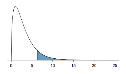
Figure B.4.7(a) shows a chi-square distribution with 3 degrees of freedom and an upper shaded tail starting at 6.25. Use Figure B.4.1 to estimate the shaded area.
This distribution has three degrees of freedom, so only the row with 3 degrees of freedom (df) is relevant. This row has been italicized in the table. Next, we see that the value 6.25 falls in the column with upper tail area 0.1. That is, the shaded upper tail of Figure B.4.7(a) has area 0.1. This example was unusual, in that we observed the exact value in the table. In the next examples, we encounter situations where we cannot precisely estimate the tail area and must instead provide a range of values.
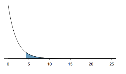
Figure B.4.7(b) shows the upper tail of a chi-square distribution with 2 degrees of freedom. The area above value 4.3 has been shaded; find this tail area.
The cutoff 4.3 falls between the second and third columns in the 2 degrees of freedom row. Because these columns correspond to tail areas of 0.2 and 0.1, we can be certain that the area shaded in Figure B.4.7(b) is between 0.1 and 0.2.
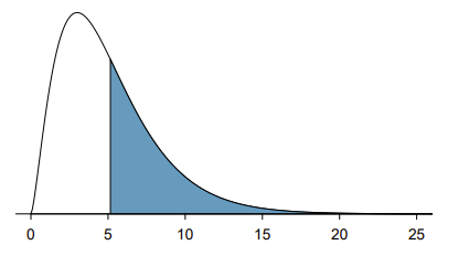
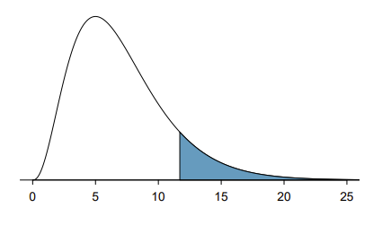
FigureB.4.7.(a) Chi-square distribution with 3 degrees of freedom, area above 6.25 shaded. (b) 2 degrees of freedom, area above 4.3 shaded. (c) 5 degrees of freedom, area above 5.1 shaded. (d) 7 degrees of freedom, area above 11.7 shaded